CalLibrary Overview

Originally written by Stewart Williams (UKATC).

An overview of the callibrary module and how it tracks calibration state.

Purpose and Introduction

The callibrary module (pipeline.infrastructure.callibrary) provides a system for managing calibration data and its application to measurement sets. It serves as the calibration management backbone of the pipeline, tracking which calibration tables should be applied to which datasets and with what parameters.

The purpose of this document is to give an overview of the callibrary module and the core concepts involved with calibration management in the pipeline.

Core Concepts

The pipeline’s callibrary is a pipeline data store that, as its input, accepts registrations of calibration tables associated with specific data selections. As output, it provides functions to retrieve the current calibration state for any selection – which may be different from the original registration – formatted as CASA preapply arguments or as permanent applycal commands.

When calibrations are applied via a CASA applycal command, the measurement set on disk is permanently modified. In contrast, CASA’s “preapply” functionality applies calibration tables in memory during CASA task execution, leaving the original measurement set untouched. This enables temporary application of calibrations that can be discarded or replaced as improved solutions are derived, all while minimising I/O and leaving the input measurement set in its pristine original state.

Input and output to the callibrary is built around three fundamental concepts:

• CalTo represents a target data selection to which calibrations should be applied

• CalFrom represents a calibration table and its application parameters

• CalApplication links calibration tables (CalFrom) to target data selections (CalTo)

Data Selection (CalTo)

The CalTo class defines what data should have calibrations applied to it, with parameters including:

• Measurement set (vis)

• Field(s), given as field name or field ID

• Spectral window(s) (spw)

• Antenna(s), given as antenna name or ID

• Observing intent(s), given in pipeline form, not as a CASA intent

Calibration Sources (CalFrom)

The CalFrom class defines a calibration table and how it should be applied. It maps to the preapply parameters of CASA calibration tasks, holding information for:

• Calibration table filename (gaintable)

• Field(s) to select from calibration table (gainfield)

• Interpolation method (interp)

• Spectral window mapping (spwmap)

• Weight application (calwt)

• Calibration type (caltype)

Calibration Application (CalApplication)

A CalApplication object connects CalTo and CalFrom objects, defining which calibrations apply to a certain data selection.

During pipeline execution, multiple calibration tables are generated and registered with the CalLibrary. By the time the h_applycal task is run, a specific data selection may have multiple calibration tables registered against it, each table requiring different application parameters. For example, the CalApplication for the PHASE calibrator with field ID #3 in spectral window 17 (i.e., CalTo has values spw=17, field=3, intent='PHASE') might reference multiple CalFrom instances. Each CalFrom instance specifies how to apply a particular calibration table to that data – such as applying a phase-up table with parameters P1, a bandpass table with parameters P2, and a Tsys table with parameters P3.

Each CalApplication holds enough information to be converted into an equivalent CASA applycal command that would permanently apply the calibration to the data. The CalApplication.as_applycal() method returns a string representation of this command. While this string form is now mainly used for exporting callibrary state, it remains a useful, human-readable format for debugging or inspecting calibration state.

Calibration State

The callibrary module has two primary data structures, one for holding aggregated calibration state and for managing instances of this state:

• CalState represents the aggregate calibration state of some data handled by the pipeline. It can represent a range of calibration targets, from the full aggregate state of every measurement set registered with the pipeline, to calibrations applying to one small part of one measurement set.

• CalLibrary is the root object for pipeline calibration state, holding active and applied calibration state and presenting methods to operate on that state.

CalState

CalState tracks which calibrations apply across the different axes of a measurement set (such as spectral window, antenna, intent, etc.). The CalState is capable of recording a unique set of calibrations and caltable application parameters for every unique permutation of measurement set, field, spectral window, observing intent, and antenna.

In essence, CalState records which CalFrom objects should be applied to each target data selection. However, the CalState is not simply a list of CalApplications, nor does it use CalTo objects to represent target data selections. Instead of CalTos, it employs a more efficient data structure based on interval trees to give better scalability[1].

That said, the overall state represented by a CalState can conceptually still be viewed as a list of CalApplications, and methods are provided to generate this convenient “list of CalApplications” representation (see IntervalCalState.merged() and expand_calstate()).

CalLibrary

CalLibrary manages the evolving calibration state throughout a pipeline run. Every pipeline Context has one instance of a CalLibrary, stored at the context.callibrary field.

As calibration tasks execute, new calibrations are registered using the CalLibrary.add() method (e.g., via context.callibrary.add()). These updates populate the active calibration state (specifically, the active CalState held by the context’s callibrary instance) which is used for all pre-apply calibration and the final applycal calls. As the pipeline state is always restored at the end of a task, and the pipeline context is only mutated when accepting results – which includes any permanent manipulation of calibration state – tasks can freely add and remove calibrations to context.callibrary during task execution without permanently affecting state.

When calibrations are permanently applied via h_applycal, the applied state is removed from the active state using CalLibrary.remove() and added to the applied calibration state (the CalLibrary.applied field, available at context.callibrary.applied). This applied state is later referenced by h_exportdata, where its .as_applycal() representation is written to disk, providing the final set of calibrations required to restore calibration to a pristine measurement set.

Note that some calibrations remain in the CalLibrary.active CalState even after h_applycal has executed. This occurs because certain registrations cover broad portions of the measurement set, while the final applycal call makes a narrower data selection (e.g., only science spectral windows). Any remaining state in .active is harmless and simply reflects h_applycal being selective about which data is permanently calibrated.

Historical Context

For many years, CASA did not include a callibrary implementation. Calibration pre-apply parameters had to be specified directly in CASA task calls, which allowed only one set of parameters per call. Since different data selections often require different pre-apply parameters, this typically resulted in a single pipeline task executing multiple CASA calls for a single conceptual task – each CASA call corresponding to a unique calibration parameter set. Minimizing the number of CASA calls was critical because every call required a traversal of the measurement set, compounding the problem of disk I/O being the main bottleneck of the calibration pipeline.

Hence, simply registering calibrations to data selections was not enough; the overall calibration state had to be optimised to minimise the number of CASA calls. This requirement led to the development of the CalLibrary and CalState, which could combine and “defragment” registered calibrations to give the smallest possible number of pre-apply states. The number of pre-apply states required depends on the target data selection, so this optimisation is done at runtime, when the pipeline knows which data the task will process.

The original CalLibrary implementation in the pipeline used deeply nested Python dictionaries (e.g., calstate[spw][field][intent][ant]) to map calibrations to data selections. This implementation was effective for ALMA data and used in early ALMA observing cycles. However, when EVLA adopted the ALMA pipeline framework, it was found that the dictionary-based implementation did not scale well to EVLA dimensions, where reduction of some datasets would exhaust the available memory.

To address this, a more memory-efficient solution using interval trees was introduced. It was designed to be interface-compatible with the original dict-based CalLibrary implementation, and for a time, both implementations coexisted in the pipeline. The callibrary.CalLibrary and callibrary.CalState aliases could point to either implementation as needed. For many years, the CalLibrary alias has pointed to the IntervalCalLibrary, though the legacy DictCalLibrary remains visible in the commit history.

With CASA’s native callibrary now available, the pipeline’s calibration state can now be exported to CASA callibrary format, allowing CASA to import it and execute one task per measurement set. This reduces the need for an optimised CalLibrary state. However, the optimised representation remains valuable for weblog tables and for import/export operations, where the unoptimised state proves difficult to interpret.

Key Features

Interval Tree State Representation

The callibrary module uses interval trees to efficiently represent multi-dimensional data selections. Interval trees compactly represent ranges, reducing memory requirements. For example, the range [1,2,3,4,5] can be represented with one interval tree containing an interval range 1–5, rather than requiring five instances. Operations on interval trees (like finding overlaps or merging) are typically \(O(\log n)\) rather than \(O(n)\), significantly improving performance for large datasets. Interval trees also allow efficient intersection, union, and containment operations on ranges of values, which assists with state arithmetic.

It is important to note that interval ranges are contiguous numerical ranges, e.g., ant=0-16, spw=3-5. Numerical interval ranges map naturally to antenna, spectral window, and field, since their CASA IDs are already numeric and can be used directly.

However, scan intent in CASA is represented as strings, not numbers. To handle this, CalState defines its own mapping from string intents to numeric IDs, allowing scan intent ranges to be represented in interval trees just like the other dimensions.

The classes CalToIntervalAdapter and CalToIdAdapter manage conversion automatically, translating between string scan intents, field names, and their corresponding interval tree IDs.

An interval range stores a value that applies to specific ranges. For example, the range 1–5 might store the value 'hello' – or it could point to another interval tree. In the CalState, each attribute from a CalTo (like antenna, spectral window, field, and intent) is represented using four levels of nested interval trees – one for each dimension of a measurement set.

• The first level (e.g., antenna range 1–42) points to a second-level interval tree.

• The second level (e.g., spectral window range 1–16) points to a third-level tree.

• The third level (e.g., field range 1–3) points to a fourth-level tree.

• The fourth level (e.g., intent range 'PHASE,BANDPASS') contains the actual CalFroms – the calibration data that applies to that full combination of antenna, spw, field, and intent.

When initializing a new CalState for a measurement set at the start of a pipeline run, the CalLibrary determines the maximum ranges needed for each dimension – antenna, spectral window, field, and intent – across all measurement sets in the session. It then sets up the interval tree data structures accordingly.

The example data structure below illustrates this setup, albeit simplified slightly for brevity. In practice, the id_to_intent mapping is also organized by measurement set name, allowing intent strings to be correctly resolved per measurement set.

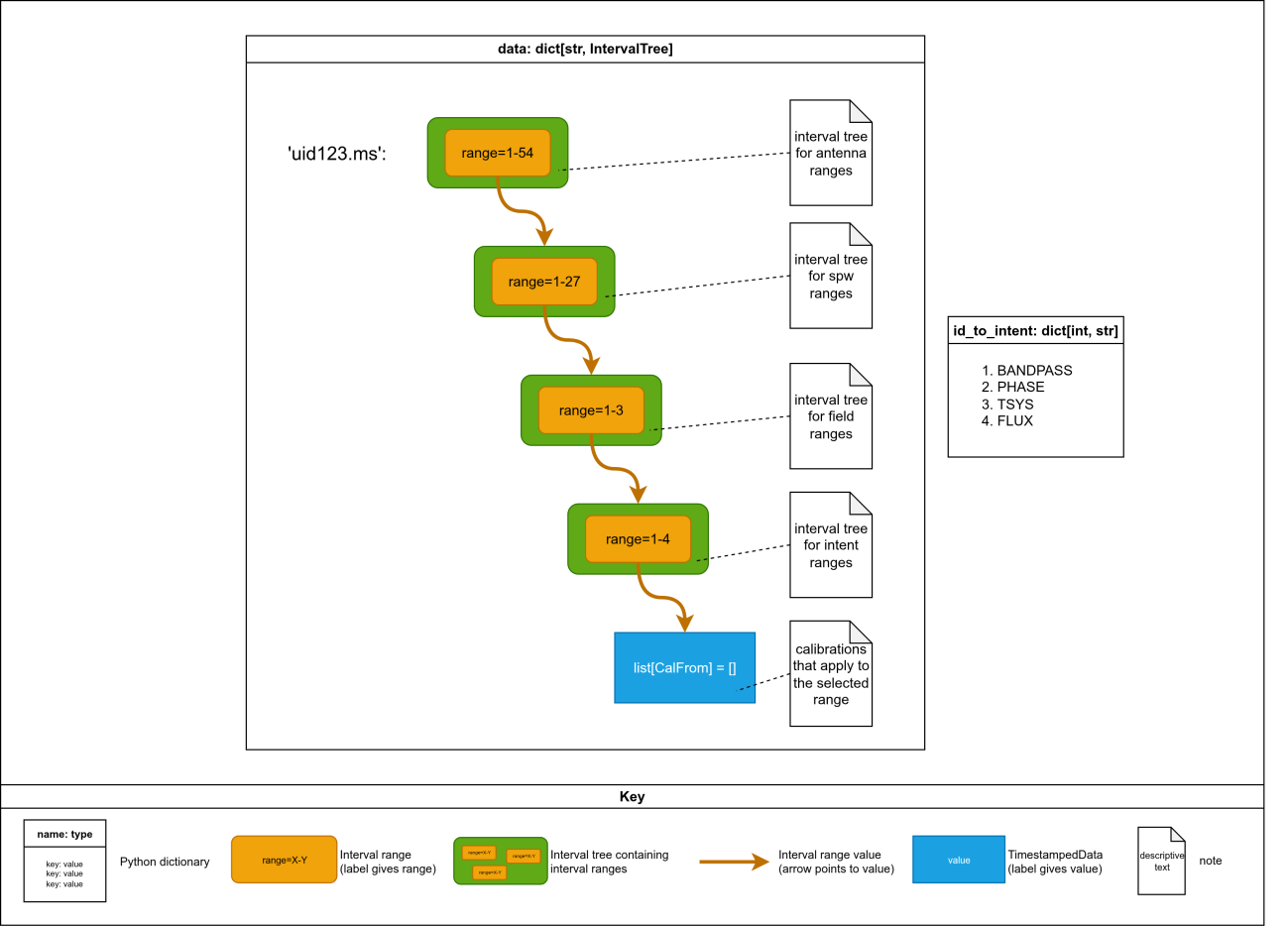
Example CalState interval tree data structure showing the four levels of nested interval trees (antenna → spectral window → field → intent) with CalFrom values at the leaves.

Note that each ant, spw, and field interval range points to a new interval tree instance. Adding fine-grained calibrations can quickly fragment the data structure, with many new interval trees and interval ranges created to accommodate calibration registration to the partial data selection. For example, starting with a pristine CalState and registering a caltable to exactly one antenna, say antenna 10, results in the root data structure being bifurcated three ways:

1. The original interval range being trimmed to antennas 0 to 9.

2. A new interval range hierarchy being created for antenna 10, with new interval trees and interval ranges for spw, field, and intent, with a final value extended to hold the new caltable.

3. A new interval range being created for antennas 11 onward, again with new interval trees instances and ranges created for spw, field, and intent, but with final value equal to the original tree.

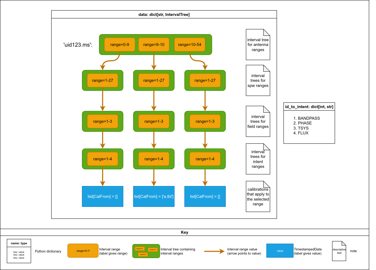
Interval tree bifurcation after registering a caltable to antenna 10. The original single antenna range is split into three ranges (0–9, 10, 11+), each with its own sub-tree hierarchy.

This simple operation roughly tripled the CalState’s memory consumption and the processing time required to operate on it! The number of interval trees and interval ranges needed to represent a calibration state can be minimized by ordering the dimensions based on how likely each axis is to be selected by pipeline tasks. Currently, the interval tree hierarchy follows this order: antenna → spectral window → field → intent – reflecting the typical targeting patterns in the pipeline calibration stages; calibrations are (almost) never applied to specific antenna, but application of caltables just to 'PHASE' or 'BANDPASS' intent, etc., is commonplace.

This order could, in principle, be changed if calibrations focus and select more on the higher levels of the hierarchy. For example, if fine-grained calibrations frequently target specific antennas more than they do specific intents, the hierarchy could be adjusted accordingly.

Note that some data selection axes such as polarisation, scan, and timerange are not currently included in the interval tree structure, as these axes have not been selectively targeted by pipeline calibration tasks. However, supporting selection and calibration application via these axes would be possible, beginning by adding new CalTo fields and adding a new level to the interval tree function chains, first in the create_interval_tree_for_ms function:

tree_intervals = [
    [(0, len(ms.intents))],
    [get_min_max(ms.fields, keyfunc=id_getter)],
    [get_min_max(ms.spectral_windows, keyfunc=id_getter)],
    [get_min_max(ms.antennas, keyfunc=id_getter)]
]

…but also in the CalState arithmetic chains, defined at the module level:

# this chain of functions defines how to add overlapping Intervals when adding
# IntervalTrees
intent_add: Callable = create_data_reducer(join=merge_lists(join_fn=operator.add))
field_add: Callable = create_data_reducer(join=merge_intervaltrees(intent_add))
spw_add: Callable = create_data_reducer(join=merge_intervaltrees(field_add))
ant_add: Callable = create_data_reducer(join=merge_intervaltrees(spw_add))


# this chain of functions defines how to subtract overlapping Intervals when
# subtracting IntervalTrees
intent_sub: Callable = create_data_reducer(join=merge_lists(join_fn=lambda x, y: [item for item in x if item not in y]))
field_sub: Callable = create_data_reducer(join=merge_intervaltrees(intent_sub))
spw_sub: Callable = create_data_reducer(join=merge_intervaltrees(field_sub))
ant_sub: Callable = create_data_reducer(join=merge_intervaltrees(spw_sub))

State Consolidation and Optimisation

The system consolidates (or “defragments”) overlapping data selections that apply the same calibration to minimize the number of calibration applications.

For example, CalTo instances for spw=1, spw=2, spw=3, and spw=9 that apply the same caltables in the same way (i.e., they have the same CalFroms) can be consolidated into two interval ranges, one covering spw=1-3, and one covering spw=9. A further round of consolidation is applied when exporting to CalApplications or applycal statements as, unlike interval ranges where the range must be contiguous, CASA ranges can be disjoint (e.g., '1,5,8-10,11-52').

The consolidate_calibrations function analyzes data selections with identical calibration requirements and merges them when possible. The actual implementation is more complicated than the example above as it must evaluate and consider each level of the interval tree chain, but the principle remains the same. It works by grouping calibrations by measurement set, then checking if merged data selections would conflict with other registered calibrations. This consolidation can reduce thousands of calibration applications to a few dozen, dramatically improving pipeline performance.

Memory Optimization with Flyweight Pattern

Many thousands of CalFroms are logically represented per CalState: one CalFrom instance per combination of measurement set, spectral window, field, antenna, and intent. Most CalFroms represent a small set of identical caltable applications. The Flyweight design pattern is used to significantly reduce the memory consumption of these “identical” CalFroms by reusing existing identical objects rather than creating duplicates, which would otherwise consume excessive memory.

The class uses a module-level weak reference dictionary to store unique instances. When creating a new CalFrom, the system first checks if an identical one already exists in the pool. To make this pattern work, CalFrom objects are designed to be immutable. Properties are accessed via getters, and there are no setters.

CalState Arithmetic

The CalState class implements Python addition and subtraction arithmetic operators to allow intuitive operations on calibration state.

Calculating a new aggregate calibration state can be coded as simply as final_state = old_state + new_state. Similarly, calculating a residual state after application of calibrations can be coded as pending_calibrations = active_calibrations - applied_calibrations.

The CalState arithmetic operations are used internally by the CalLibrary to manipulate calibration state. The CalLibrary.add() method used to register new calibrations becomes:

def add(self, calto, calfroms):
    to_add = IntervalCalState.from_calapplication(self._context, calto, calfroms)
    self._active += to_add

While the CalLibrary method used after applycal to deregister calibrations and mark them as part of the historical “applied” state is:

def mark_as_applied(self, calto, calfrom):
    application = IntervalCalState.from_calapplication(self._context, calto, calfrom)
    self._active -= application
    self._applied += application

Making arithmetical operators work correctly requires some additional CalLibrary machinery.

The code wraps list of CalFroms in a TimeStampedData object, which is a namedtuple that adds a timestamp and UUID marker to the values held by the interval ranges.

Identical calibrations have the same hash and would be treated as duplicates in set operations, leading to incorrect results when performing arithmetic operations. To prevent this, the callibrary temporarily marks one operand with a UUID to ensure proper distinction during processing.

The timestamp in a TimestampedData is used to sort the data fields, thus ensuring that the addition of two CalStates gives the expected result, regardless of operand order. Specifically, the timestamps ensure that caltables are ordered chronologically, so that later pipeline stages append their caltables to the end of the current caltable list. See callibrary.create_data_reducer as an entry point into this code.

Dual Modes: Integrate with CASA CalLibrary, or Split into Jobs

Pipeline tasks can export an applicable pipeline CalState as a text file in CASA callibrary format. This file can be used as input to CASA tasks that are CASA callibrary capable, allowing data with disjoint calibration states and data selections to be calibrated in one CASA call.

Alternatively, pipeline tasks can request the callibrary to split the calibration (pre)application into the required number of CASA tasks, each task specifying its own unique set of data selection and calibration parameters.

Ideally, all calibrations would use the CASA CalLibrary, both for pre-applying calibrations and for their permanent application. However, not all calibration tasks and states can be applied with the CASA CalLibrary[2]. Consequently, all pipeline tasks – except one – continue to split task execution into multiple jobs, one job per unique calibration state.

The exception is Applycal, which switches mode depending on the calibration state to be applied: by default, the task will export the pipeline callibrary and run a single CASA applycal job that applies the exported callibrary file (see Applycal.jobs_with_calapply). However, if the calibration state includes a uvcont table or the user has explicitly set the DISABLE_CASA_CALLIBRARY[3] environment variable to True, then calibrations will be applied via multiple jobs.

Export/Import Functionality

The CalLibrary handles serialization and deserialization of calibration states by converting them into a minimal set of equivalent CASA applycal commands. This allows the pipeline’s active calibration state to be exported as a human-readable, editable, and directly executable text file, or for such a file to be imported and appended.

This design enables users to inject custom calibrations and calibration tables into the pipeline via an export/import workflow: the pipeline’s calibration state can be exported to disk, modified by the user, and then re-imported at the appropriate stage.

For more details, see the callibrary methods CalLibrary.import_state() and CalLibrary.export(), and the corresponding pipeline tasks h_import_calstate and h_export_calstate.

Querying and Trimming Calibration State

Querying calibration state and trimming the state to match the task input parameters ensures that the pipeline only applies calibrations where required. The method CalState.trimmed() creates a subset of the CalState with interval trees trimmed to match specified ranges (e.g., antennas 1–3, spw 0). The new CalState containing only relevant intervals is suitable for subsequent pipeline processing.

The method CalLibrary.get_calstate() uses the CalState.trimmed() function internally. The get_calstate method can also mask properties (e.g., intent) of the CalFrom calibration application when constructing the trimmed CalState, allowing fine-grained applications to be broadened in the query result.

Utility Functions

A functional approach was taken for the core CalLibrary development, and so much of the code that operates on state exists as module-level functions. The module includes numerous utility functions for:

• Converting between CASA and internal representations

• Managing interval trees

• Consolidating calibrations

• Handling special cases (e.g., Cycle 0 data)

These functions are called by the CalLibrary and CalState classes as required to operate on their state.

Integration Points

The callibrary depends on:

• Pipeline context and MeasurementSet domain objects

  Domain objects attached to the MeasurementSet objects are used to populate the dicts that map string values for field and intent to the numerical IDs used in the interval ranges.

  Domain objects are also inspected to determine the appropriate interval ranges when initialising a CalState. The interval trees in a calstate are populated with interval ranges set to match the extent of each measurement set axis, e.g., antenna range of 1–48, spw range of 1–32, etc.

• Table reader

  Table reader is used to determine the caltable type as it is registered. This information is used to return caltables of the appropriate type when tasks query the active calibration state.

Common Workflows

Pre-applying Calibrations by Splitting into Jobs

To apply the appropriate pre-apply parameters for a CASA task, the general workflow is:

1. Retrieve relevant calibrations for a data selection.

2. Iterate over the distinct CalApplications returned by CalState.merged().

3. For each distinct CalApplication, read the CalTo and CalFrom values from the CalApplication and set the CASA task’s preapply arguments accordingly.

4. Execute the CASA task for the unique calibration state using the task executor.

This remains the dominant pre-apply workflow in the pipeline. Examples include GaincalWorker.prepare(), BandpassWorker.prepare(), and PolcalWorker.prepare().

Pre-Applying Calibrations using the CASA CalLibrary

To apply the appropriate pre-apply parameters for a CASA task using the CASA CalLibrary, the workflow is:

1. Retrieve relevant calibrations for a data selection.

2. Export the pipeline calibration state in CASA callibrary syntax.

3. Apply the CASA callibrary state to the CASA task.

Only one example exists of this workflow: SerialApplycal.prepare(). Note that the mode may switch to splitting into jobs, depending on presence of uvcont tables in the calibration state. See the section on dual modes for more details.

Permanently Registering New Calibrations

Registering new calibrations is common to many pipeline calibration tasks. The workflow is:

1. Create a CalTo object defining the target data.

2. Create CalFrom object(s) for calibration table(s) to apply.

3. Make a record of these CalApplications on the task result.

4. In the task result’s merge_with_context() method, add the CalApplications to the context’s active calibration state.

For examples of this workflow, see GaincalWorker.merge_with_context() and TsyscalResults.merge_with_context(). Both of these classes construct a CalApplication representing the desired final calibration during task execution, with the main calibration state only permanently modified during results acceptance.

Pipeline tasks that permanently register new calibrations include:

• h_tsyscal: registers the Tsys calibration table.

• hif_antpos: registers the antenna position correction table created by CASA gencal.

• hifa_bandpass: registers the bandpass calibration table.

• hifa_diffgaincal: registers the diffgain on-source phase caltable.

• hifa_polcal: registers the XY delay, XY phase, leakage term, XY ratio, and amplitude caltables for polarization calibrator.

• hifa_renorm: registers the renormalization caltable.

• hifa_spwphaseup: registers a spw-to-spw phase offsets caltable.

• hifa_timegaincal: registers phase and amplitude caltables.

• hifa_wvrgcal: registers the WVR gain table.

• hifv_circfeedpolcal: registers the polarization caltable for VLA circular feeds.

• hifv_finalcals: registers the final calibration tables to be applied to the data in the VLA CASA pipeline.

• hifv_priorcals: gaincal curves, opcal, requantizer gains, switched power cal.

• hsd_k2jycal: Kelvin to Jansky caltable.

Processing a Caltable Generated by a Previous Stage

Some pipeline tasks need to process a calibration table generated by a previous pipeline stage. All information transfer between pipeline stages is achieved via the context, hence the context must be queried for the information on the caltable registration in question. For caltable post-processing, just the filename is required.

The recommended workflow for operating on a caltable from a previous stage is:

1. Add a caltable field to the task Inputs, with default value populated by a get_caltable() call on the active CalState.

2. In the task prepare() method, read the inputs field and process the caltable.

TsysflagInputs is a good example of this flow, where the Tsys table created and registered in a prior Tsyscal stage is retrieved by its table type. In the task, the Tsys table is then processed and flagged but no new caltable registration is required, as the modifications are made to a table already registered with the pipeline. Other examples of this workflow are TsysflagContaminationInputs and SDATMCorrectionInputs.

Some tasks access calibration tables during execution or QA steps but do not expose the table as an input (i.e., they skip step 1), hence they do not allow any way for the user to override the caltable being processed or analysed. Examples include: AtmHeuristics, SDImaging, BPSolInt, and QA processing for hifa_fluxscale.

Temporarily Modifying Calibration State Within a Task

Several tasks need to temporarily add, replace, or remove caltables from the calibration state during task execution, without making these modifications permanent. The workflow for these operations is:

1. In the main body of the pipeline task – but before running the pipeline child task in question – create CalApplications that specify how the pipeline should be temporarily modified.

2. For the addition of new caltables:

   • Register the new CalApplications with the context.active state prior to CASA task or child pipeline task execution.

3. To temporarily remove caltables:

   • Create a predicate function that identifies the caltable to temporarily remove. For example:

     def match_tsys(calto, calfrom):
         return calfrom.type == 'tsys'
     

   • Call CalLibrary.unregister_calibrations(), passing in the predicate function.

4. To replace a caltable, perform steps 2 and 3 together.

5. Run the child pipeline task using the pipeline executor.

This workflow takes advantage of the pipeline architecture whereby tasks operate on a clone of the context, and not the master copy. As such, they are free to modify the calibration state at will.

Tasks that temporarily register calibrations within the task include:

• hif_lowgainflag: creates and registers temporary bandpass, phase, and amplitude caltables prior to flagging heuristic.

• hif_selfcal: registers self-cal gain table locally prior to permanently applying this to MS.

• hifa_bandpass: creates a temporary spw-to-spw phase offset caltable that is subsequently used during bandpass step.

• hifa_bandpassflag: creates temporary phase caltable and a temporary bandpass to context, prior to amplitude solve and applycal and subsequent corrected amp flagging heuristic.

• hifa_gfluxscale: creates temporary phase caltables and registers those in local context prior to subsequent amplitude gaincal step; temporarily unregisters amplitude caltable from local context and registers temporary fluxscale created caltable prior to the step computing the calibrated visibility fluxes (which starts with an applycal step).

• hifa_gfluxscaleflag: creates and registers temporary phase and amplitude caltables before running an applycal and subsequent corrected amp flag heuristic.

• hifa_polcal: makes significant use of temporarily registering caltables as well as unregistering caltables at certain points.

• hifa_polcalflag: creates and registers temporary phase and amplitude caltables before running an applycal and subsequent corrected amp flag heuristic.

• hifa_timegaincal: temporarily registers phase cal table prior to computing amplitude caltable; unregisters phasecal-without-combine when applicable, and re-registers in local context a phasecal-with-combine before computing diagnostic residual phase offset caltable.

• hifa_wvrgcal: in its “analyse” step, if it cannot find a suitable bandpass (seemingly fed in through inputs), it will invoke hifa_bandpass locally and register that bandpass table in local context to use in pre-apply during subsequent processing.

• hsdn.tasks.restoredata.ampcal.SDAmpCal: used by hsdn_restoredata to register an amplitude scaling prior to its applycal step.

Permanently Removing Calibrations from the Calibration State

Once calibrations are applied, they need to be permanently removed from the calibration state – otherwise they would continue to be pre-applied in any subsequent stage that uses calibration tasks.

For the case of applying calibrations, the workflow for applying and then permanently removing them from the calibration state is:

1. If desired, permanently apply the pipeline callibrary state to the target dataset (see applycal workflow above).

2. In that task Result’s merge_with_context() method, remove the applied calibrations from the active calibration state.

For an implementation of this workflow, see ApplycalResults.merge_with_context(). Note that removing calibration state from the active state adds it to the context.callibrary.applied state, retaining a history of how the calibration state came to be.

Managing Calibration State

Export/import calibration state

As a developer, calibration state can be exported to and imported from a text file via CalLibrary.export() and CalLibrary.import_state() methods, respectively. These functions write the state in CASA applycal format, which is usually the most appropriate format when developing pipeline tasks.

The debugging helper method _print_dimensions() can also be useful when debugging CalState internals, where it can be used to inspect interval ranges directly.

Clear calibration states

context.callibrary.active.clear() and context.callibrary.applied.clear() clear the active and applied calibration states, respectively. Used in conjunction with import and export state functions, this can be useful for priming the pipeline context with a pre-prepared state ahead of tests.

Future Improvements

The consolidate_calibrations() function can be the slowest operation in the CalLibrary, and could potentially be optimised. The current implementation is a bottleneck because it iteratively merges data selections (CalToArgs) that share the same calibration application (list of CalFrom objects), performing repeated conflict checks that can be computationally expensive, especially with a large number of selections.

The function takes a list of (CalTo, [CalFrom]) tuples. The goal is to consolidate these tuples by merging CalToArgs that have identical [CalFrom] lists (same calibration application) into fewer entries, combining their data selections (e.g., union of antenna sets), provided the merged selection doesn’t overlap with selections tied to different calibrations. Overlap occurs if two CalToArgs share at least one element in each dimension (vis, antenna, field, spw, intent).

The current process:

1. Groups by MS: Partitions tuples by their measurement set (vis).

2. Hashes CalFrom Lists: Creates a unique hash for each [CalFrom] list to group CalToArgs with the same calibration.

3. Iterative Merging: For each group, iteratively attempts to merge each CalToArgs with existing merged selections, checking for conflicts with selections having different calibrations. If no conflict, it merges; if a conflict exists, it keeps them separate.

The inefficiency lies in the iterative merging and conflict checking. For each CalToArgs in a group:

• It tries to merge with each existing merged selection.

• For each merge attempt, it checks if the proposed merged selection overlaps with all selections having different calibrations (other_data_selections).

This involves set intersection checks across multiple dimensions, repeated for every merge attempt. A more efficient strategy that avoids iterative merging could be:

1. Identify all CalToArgs with the same calibration that can be merged safely in one pass.

2. Merge them at once, reducing redundant conflict checks.

---

[1]

See section on Interval Tree State Representation.

[2]

This was the case in 2019, because CASA callibrary did not support all the pre-apply parameters offered by CASA tasks used by the pipeline. Specifically, the CASA callibrary did not support the gainfieldmap argument, and was incapable of pre-applying calibrations that reference multiple fields. CASA’s CalLibrary implementation may have matured since then.

[3]

This environment variable was introduced as a feature flag during initial pipeline integration with CASA callibrary, allowing integration to be disabled should issues arise. It is likely that this variable is now redundant and could be removed.