hsd_baseline

hsd_baseline(fitfunc: FitFunc | None = None, fitorder: FitOrder | None = None, switchpoly: bool | None = None, linewindow: LineWindow | None = None, linewindowmode: str | None = None, edge: tuple[int, int] | None = None, broadline: bool | None = None, clusteringalgorithm: str | None = None, wave_number: list[int] | None = None, deviationmask: bool | None = None, deviationmask_sigma_threshold: bool | None = None, parallel: str | None = None, infiles: list[str] | None = None, field: list[str] | None = None, antenna: list[str] | None = None, spw: list[str] | None = None, pol: list[str] | None = None) → SDBaselineResults

Detect spectral line features and subtract the baseline from calibrated single-dish spectra.

Generates baseline fitting tables and subtracts the baseline from the spectra by masking detected emission/absorption line regions. The WebLog shows three sections of spectral grid maps per source:

1. Spectra before baseline subtraction (red fitted curve overlaid on each grid cell).

2. Averaged spectra per grid cell (improves S/N to reveal line features).

3. Spectra after baseline subtraction (red line at zero level per grid cell).

Cyan-shaded regions indicate the sum of all emission-line channels identified across the entire map (not just the individual grid cell). A spatially integrated spectrum per ASDM, antenna, spw, and polarization is shown above each grid, with the magenta curve indicating atmospheric transmission and thick red bars marking channels excluded by the deviation mask algorithm. Representative spectra in each cell correspond to the valid pointing nearest the mean coordinates of all pointings in that grid cell.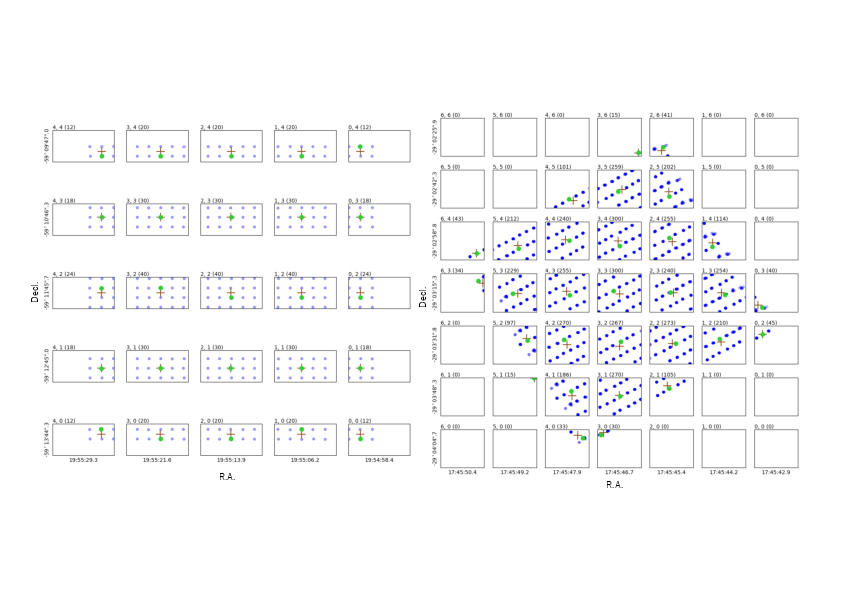

Examples of how representative positions are determined. Blue points are all pointings; brown crosses are the averaged coordinates; green circles mark the representative positions (nearest valid pointing to the averaged coordinates).

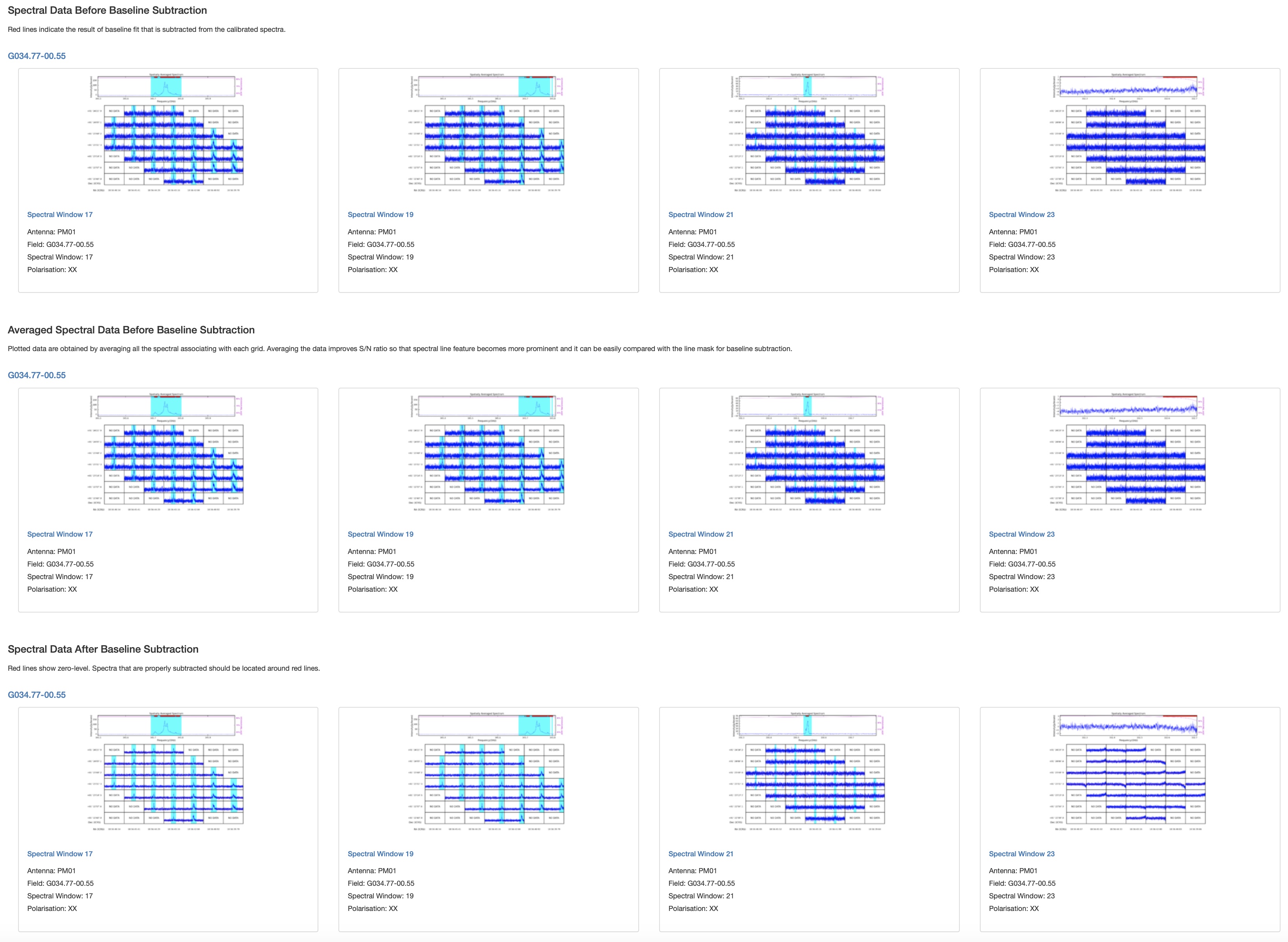
Example of the hsd_baseline WebLog page showing the first three spectral grid rows (before subtraction, averaged, after subtraction) for one spw.

Detailed per-antenna spectral maps can be accessed from the detail pages by clicking the Spectral Window link on each summary page. Filters by antenna, field, spectral window, and polarization are available in the upper part of the detail pages.

Fitting order determination: The default function is a cubic spline. The number of spline segments (N_segment) is determined via FFT analysis of the power spectrum of grouped spectra:

1. 1 < P_FFT < 3 -- N_segment = 4

2. 3 <= P_FFT < 5 -- N_segment = 5

3. 5 <= P_FFT < 10 -- N_segment = 6

4. P_FFT >= 10 -- N_segment = F_FFT * 2 + 2

The final N_segment is scaled by (Nch - N_mask) / Nch to account for masked channels. Specifying a non-negative integer for fitorder disables auto-determination.

Mask range determination: Emission/absorption channels are identified by comparing spectral deviation from the median against an MAD-based threshold. Up to 10 iterations are performed to detect weak lines; each detected range is extended while the intensity is monotonically decreasing/increasing. Binned spectra (widths 1, 4, 16, 64 for 4096-channel spws) are also analyzed for broad features, with threshold 3.5 + sqrt(binning_width) * MAD.

Baseline flatness evaluation (fourth section of the WebLog page): Emission-free channels are divided into 10 or 20 bins. MAX(mean) - MIN(mean) across bins is compared to the spectral rms sigma.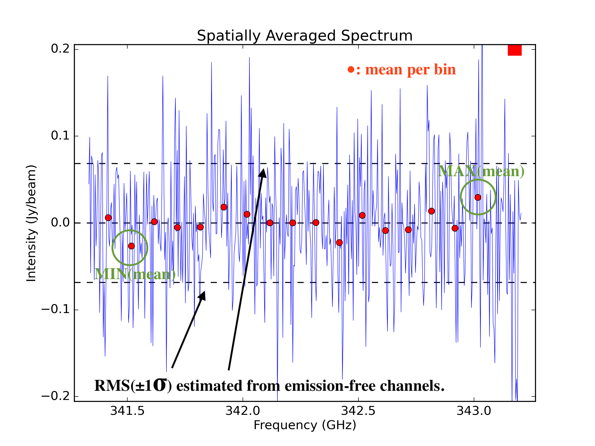

Example of baseline flatness evaluation.

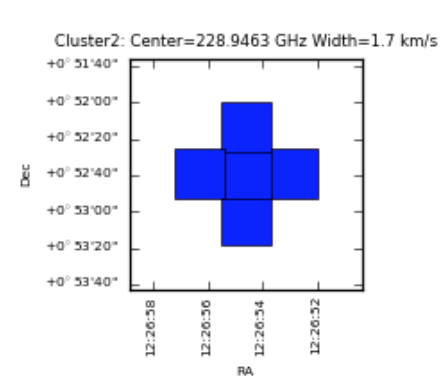
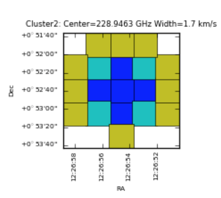
Clustering analysis for spectral line detection (developer plots, hidden by default; enable with plotlevel='all' in h_init):

Detection: grid cells with emission exceeding the threshold are identified. Yellow cells have a single time-domain group with detected emission; cyan cells have more than one.

Clustering detection step.

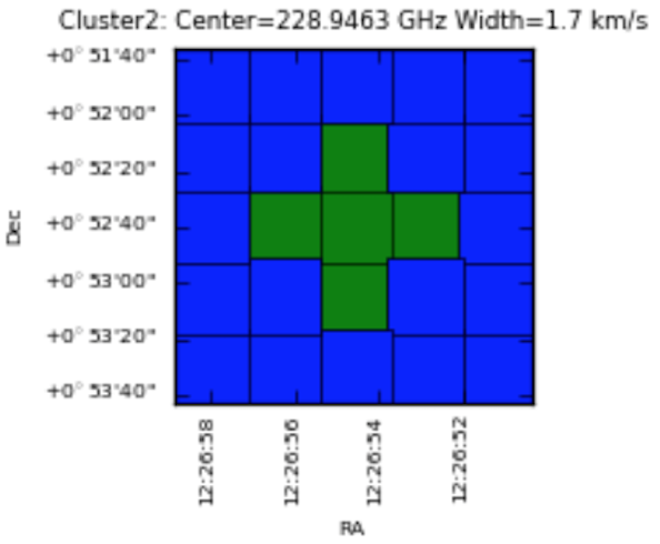
Validation: for each grid cell the ratio of spectra containing detected emission lines (Nmember) to total spectra in the cell (Nspectra) is computed:

• Validated if Nmember/Nspectra > 0.5

• Marginally validated if Nmember/Nspectra > 0.3

• Questionable if Nmember/Nspectra > 0.2

Clustering validation step.

Smoothing: the per-cell ratio is convolved with a Gaussian-like grid function to suppress isolated single-line candidates and reinforce detections supported by neighboring cells.

Clustering smoothing step.

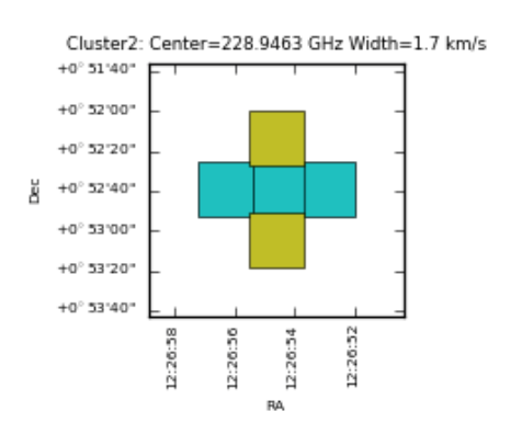
Mask region determination: in the validated area after smoothing, mask channel ranges are computed over the spatial domain by inter/extrapolating the mask ranges of the averaged spectra in validated cells and applied to each individual spectrum.

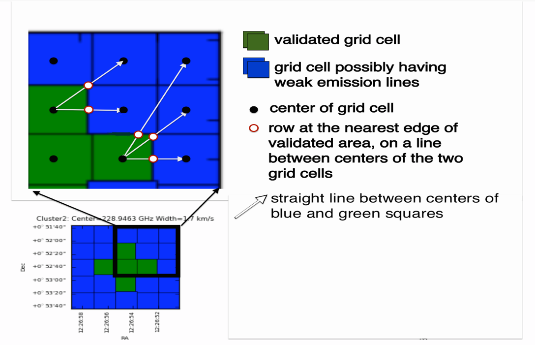
Mask range calculation — in blue squares the mask range is interpolated from validated cells.

Clustering final example.

Parameters:

• fitfunc --

  Fitting function for baseline subtraction. You can choose either cubic spline ('spline' or 'cspline'), polynomial ('poly' or 'polynomial'), sinusoid.

  Accepts:

  • A string: Applies the same function to all spectral windows (SPWs).

  • A dictionary: Maps SPW IDs (int or str) to a specific fitting function.

  If an SPW ID is not present in the dictionary, 'cspline' will be used as the default.

  Default: None (equivalent to 'cspline')

• fitorder --

  Fitting order for polynomial. For cubic spline, it is used to determine how much the spectrum is segmented into.

  Accepts:

  • An integer: Applies the same order to all SPWs. Valid values: -1 (automatic), 0, or any positive integer.

  • A dictionary: Maps SPW IDs (int or str) to a specific fitting order.

  If an SPW ID is not present in the dictionary, -1 will be used as the default, triggering automatic order selection.

  Default: None (equivalent to -1)

• switchpoly --

  Whether to fall back the fits from cubic spline to 1st or 2nd order polynomial when large masks exist at the edges of the spw. Condition for switching is as follows:

  • if nmask > nchan/2 => 1st order polynomial

  • else if nmask > nchan/4 => 2nd order polynomial

  • else => use fitfunc and fitorder

  where nmask is a number of channels for mask at edge while nchan is a number of channels of entire spectral window.

  Default: None (equivalent to True)

• linewindow --

  Pre-defined line window. If this is set, specified line windows are used as a line mask for baseline subtraction instead to determine masks based on line detection and validation stage. Several types of format are acceptable. One is channel-based window.

  [min_chan, max_chan]
  

  where min_chan and max_chan should be an integer. For multiple windows, nested list is also acceptable.

  [[min_chan0, max_chan0], [min_chan1, max_chan1], ...]
  

  Another way is frequency-based window.

  [min_freq, max_freq]
  

  where min_freq and max_freq should be either a float or a string. If float value is given, it is interpreted as a frequency in Hz. String should be a quantity consisting of "value" and "unit", e.g., '100GHz'. Multiple windows are also supported.

  [[min_freq0, max_freq0], [min_freq1, max_freq1], ...]
  

  Note that the specified frequencies are assumed to be the value in LSRK frame. Note also that there is a limitation when multiple MSes are processed. If native frequency frame of the data is not LSRK (e.g. TOPO), frequencies need to be converted to that frame. As a result, corresponding channel range may vary between MSes. However, current implementation is not able to handle such case. Frequencies are converted to desired frame using representative MS (time, position, direction).

  In the above cases, specified line windows are applied to all science spws. In case when line windows vary with spw, line windows can be specified by a dictionary whose key is spw id while value is line window. For example, the following dictionary gives different line windows to spws 17 and 19. Other spws, if available, will have an empty line window.

  {17: [[100, 200], [1200, 1400]], 19: ['112115MHz', '112116MHz']}
  

  Furthermore, linewindow accepts MS selection string. The following string gives [[100,200],[1200,1400]] for spw 17 while [1000,1500] for spw 21.

  "17:100~200;1200~1400,21:1000~1500"
  

  The string also accepts frequency with units. Note, however, that frequency reference frame in this case is not fixed to LSRK. Instead, the frame will be taken from the MS (typically TOPO for ALMA). Thus, the following two frequency-based line windows result different channel selections.

  {19: ['112115MHz', '112116MHz']} # frequency frame is LSRK
  "19:11215MHz~11216MHz" # frequency frame is taken from the data (TOPO for ALMA)
  

  None is allowed as a value of dictionary input to indicate that no line detection/validation is required even if manually specified line window does not exist. When None is given as a value and if linewindowmode is 'replace', line detection/validation is not performed for the corresponding spw. For example, suppose the following parameters are given for the data with four science spws, 17, 19, 21, and 23.

  linewindow={17: [112.1e9, 112.2e9], 19: [113.1e9, 113.15e9], 21: None}
  linewindowmode='replace'
  

  The task will use given line window for 17 and 19 while the task performs line deteciton/validation for spw 23 because no line window is set. On the other hand, line detection/validation is skipped for spw 21 due to the effect of None.

  Example: [100,200] (channel), [115e9, 115.1e9] (frequency in Hz), ['115GHz', '115.1GHz'] (see above for more examples)

  Default: None

• linewindowmode -- Merge or replace given manual line window with line detection/validation result. If 'replace' is given, line detection and validation will not be performed. On the other hand, when 'merge' is specified, line detection/validation will be performed and manually specified line windows are added to the result. Note that this has no effect when linewindow for target spw is an empty list. In that case, line detection/validation will be performed regardless of the value of linewindowmode. In case if no linewindow nor line detection/validation are necessary, you should set linewindowmode to 'replace' and specify None as a value of the linewindow dictionary for the spw to apply. See parameter description of linewindow for detail.

• edge --

  Number of edge channels to be dropped from baseline subtraction. The value must be a list with length of 2, whose values specify left and right edge channels, respectively.

  Example: [10,10]

  Default: None

• broadline --

  Try to detect broad component of spectral line if True.

  Default: None (equivalent to True)

• clusteringalgorithm --

  Selection of the algorithm used in the clustering analysis to check the validity of detected line features. The 'kmean' algorithm, hierarchical clustering algorithm, 'hierarchy', and their combination ('both') are so far implemented.

  Default: None (equivalent to 'hierarchy')

• wave_number --

  a list of sinusoidal wave numbers. The maximum wave numbers should not exceed the ((number of channels/2)-1) limit. If the offset is present in the data, add 0 to the number of waves. That is, nwave=[0] is a constant term, nwave=[0,1,2] fits with a maximum of 2 sinusoids, and so on.

  Default: None (equivalent to False)

• deviationmask --

  Apply deviation mask in addition to masks determined by the automatic line detection.

  Default: None (equivalent to True)

• deviationmask_sigma_threshold --

  Threshold factor (F) to detect the deviation. Actual threshold will be median + F * standard-deviation of the spectrum.

  Default: None (equivalent to 5.0)

• parallel --

  Execute using CASA HPC functionality, if available.

  Options: 'automatic', 'true', 'false', True, False.

  Default: None (equivalent to 'automatic').

• infiles --

  List of data files. These must be a name of MeasurementSets that are registered to context via hsd_importdata or hsd_restoredata task.

  Example: vis=['X227.ms', 'X228.ms'] Default: None (process all registered MeasurementSets)

• field --

  Data selection by field.

  Example: '1' (select by FIELD_ID), 'M100*' (select by field name), '' (all fields)

  Default: None (equivalent to '')

• antenna --

  Data selection by antenna.

  Example: '1' (select by ANTENNA_ID), 'PM03' (select by antenna name), '' (all antennas)

  Default: None (equivalent to '')

• spw --

  Data selection by spw.

  Example: '3,4' (process spw 3 and 4), ['0','2'] (spw 0 for first data, 2 for second), '' (all spws)

  Default: None (equivalent to '')

• pol --

  Data selection by polarizations.

  Example: '0' (process pol 0), ['0~1','0'] (pol 0 and 1 for first data, only 0 for second), '' (all polarizations)

  Default: None (equivalent to '')

Notes

Three QA scores are computed:

Spectral line detection:

• QA = 1.0 if no edge-line and main line is narrow.

• QA = 0.60 if no edge-line and main line is wide.

• QA = 0.55 if edge-line detected (regardless of main line width).

• QA = 0.80 if no spectral lines are detected.

• QA = 0.88 if the deviation mask overlaps with spectral or atmospheric lines.

Baseline flatness (MAX(mean) - MIN(mean) vs. sigma):

• QA = 0.33 if MAX(mean) - MIN(mean) > 3.6 sigma.

• QA = 0.33-1.0 if 1.8 sigma <= MAX(mean) - MIN(mean) < 3.6 sigma.

• QA = 1.0 if MAX(mean) - MIN(mean) < 1.8 sigma.

Deviation from zero-baseline: QA = 0.65 if significant deviation outside candidate line ranges is detected (triggering deviation masks).

Warning

hsd_baseline overwrites results from previous runs. If processing spws separately, each spw must be taken through to the imaging stage before the next spw is processed:

hsd_baseline(spw='0'); hsd_blflag(spw='0'); hsd_imaging(spw='0')
hsd_baseline(spw='1'); hsd_blflag(spw='1'); hsd_imaging(spw='1')

Returns:

The results object for the pipeline task is returned.

Examples

1. Basic usage with automatic line detection:

>>> hsd_baseline(antenna='PM03', spw='17,19')

2. Use pre-defined line windows instead of automatic detection:

>>> hsd_baseline(linewindow=[[100, 200], [1200, 1400]], linewindowmode='replace', edge=[10, 10])

3. Per-spw pre-defined line windows merged with automatic detection:

>>> hsd_baseline(linewindow={19: [[390, 550]], 23: [[100, 200], [1200, 1400]]},
...             linewindowmode='merge')