hsd_imaging
Note
Parameters set to None will use intelligent defaults from the pipeline context.
Pass explicit values to override context defaults.
- hsd_imaging(mode=None, restfreq=None, infiles=None, field=None, spw=None)[source]
Generate single-dish images per antenna and combined over all antennas.
Creates images per antenna and combined images for each field and spw. Image parameters (cell size, number of pixels, etc.) are determined automatically from metadata (antenna diameter, map extent, etc.). Images are produced in LSRK frame, or REST frame for ephemeris sources.
The WebLog for this stage includes:
Image sensitivity table: achieved rms per spw/source and theoretical rms accounting for the flagging fraction.
Profile maps: three types are shown in the WebLog — a simplified combined-image map per spw (front page), a simplified per-antenna map (click
Spectral Window), and a detailed map (one spectrum per pixel at 3-cell intervals, max 5x5 plots/page). Each spectrum in the simplified maps corresponds to the average over 1/8 of the image size, giving 8x8 spectra by default. Magenta lines show atmospheric transmission.
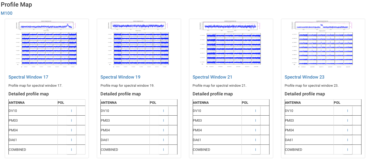
Example of the profile map.
Channel maps: one map per identified emission line per spw, showing a velocity-axis zoom of the line, the full spectral range with line width marked (red vertical lines), total integrated intensity map (Jy/beam km/s), and channel maps within the identified line velocity range (15 bins by default).
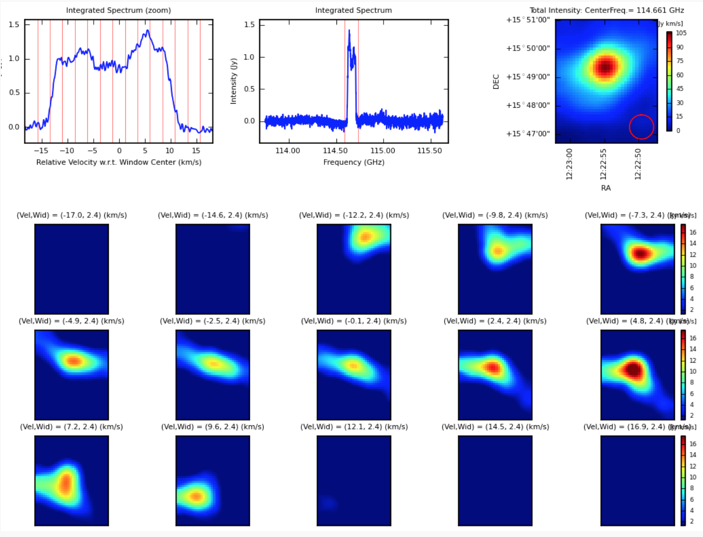
Example of a channel map.
Baseline RMS map: constructed from the baseline RMS in the baseline tables (emission-free channels); combined data only, not per antenna.
Moment maps: for each spw, three maps are generated: (1) maximum intensity map (moment-8) over all channels; (2) total intensity map (moment-0) over line-free channels; (3) maximum intensity map using line-free channels only.
Diagnostic plots for possible missed line channels (PL2025+): generated when line emission is detected outside the line ranges from
hsd_baseline(SNR threshold = 7 for "single peak" and SNR threshold = 5 for "extended").
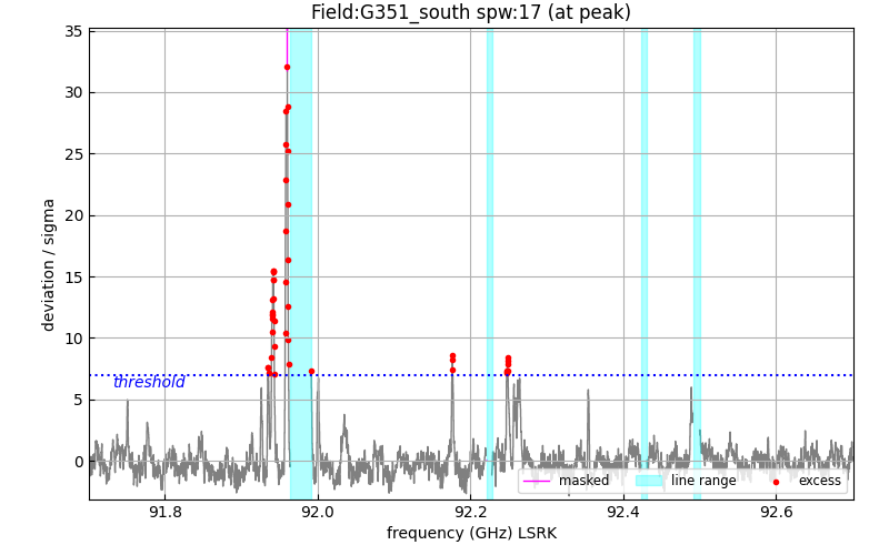
Example diagnostic plot for possible missed line channels.
Contamination plots: Peak S/N map, mask map (pixels with S/N < 10% of peak), and masked-averaged spectrum (red = masked-pixel average, grey = peak S/N position spectrum). A warning is issued if the negative peak < -4 x standard deviation.
- Parameters:
mode (str | None) --
Imaging mode controls imaging parameters in the task. Accepts either "line" (spectral line imaging) or "ampcal" (image settings for amplitude calibrator).
Default:
None(equivalent to'line')restfreq (str | None) -- Rest frequency. Defaults to None, it executes without rest frequency.
infiles (list[str] | None) --
List of data files. These must be a name of MeasurementSets that are registered to context via hsd_importdata or hsd_restoredata tasks.
Example:
vis=['uid___A002_X85c183_X36f.ms', 'uid___A002_X85c183_X60b.ms']Default:
None(process all registered MeasurementSets)field (str | None) --
Data selection by field names or ids.
Example:
"*Sgr*,M100"Default:
None(process all science fields)spw (str | None) --
Data selection by spw ids.
Example:
"3,4"(generate images for spw 3 and 4)Default:
None(process all science spws)
- Return type:
SDImagingResults
Notes
Three QA scores are computed:
Masking: QA = 1.0 if no pixels in the pointing area are masked; QA = 0.5 if any pixels are masked; QA = 0.0 if >= 10% of pixels in the pointing area are masked (linearly interpolated between 0 and 0.5).
Contamination: QA = 0.65 if possible astronomical line contamination is detected in the continuum channel selection.
Missed line channels (PL2025+): QA = 0.60 if significant off-line-range emission is detected; QA = 1.0 otherwise.
Examples
Generate images with default settings:
>>> hsd_imaging()
Generate images for the amplitude calibrator with specific parameters:
>>> hsd_imaging(mode='ampcal', field='*Sgr*,M100', spw='17,19')